As an exercise, I wrote a spiking neural network in R, implemented in a shiny app, that performs some rudimentary unsupervised learning. The app is embedded below. A small set of patterns is used to generate an input spike sequence, and a single hidden layer of spiking neurons uses a leaky integrate and fire (LIF) model with spike-timing dependent plasticity (STDP) to learn the underlying pattern components. The hidden layer uses lateral inhibition, or inhibitory connections among hidden layer neurons, to sparsify the solution. Increasing the g-bar(inh.) parameter results in stronger inhibition and less redundancy in the hidden layer. There are some difficulty settings that increase the amount of overlap between the generative patterns, and it can be seen that a single-layer network struggles to deal with that overlap.
About me:
I am passionate about understanding how the human mind works. I currently work for Astera Institute as a Senior Machine Learning Engineer developing artificial intelligence based on human cognition and neuroscience. I have previously worked as researcher in cognitive science and psychiatry. I have also worked as a statistician and methodologist for medical research generally.
New position at CCNLab
As of June 21, 2021 I have left my job as a biostatistician at Virginia Tech and joined UC Davis Computational Cognitive Neuroscience lab lab as a postdoc! I cannot express how exciting it has been to discover this kind of research but to also land an opportunity to train and do it myself. The lab has a variety of ongoing research involving biologically-constrained spiking and rate coded neural networks in the Leabra framework (github). There is an excellent textbook written and published for free online by the PI, Randy O’Reilly.
The research brings together the cellular, anatomical, statistical (information-processing), and behavioral aspects of psychology into unified theoretical models. The models simulate the tasks normally performed by human or other mammal subjects in behavioral experiments. Having worked in such labs that study various molecular and genetic aspects of schizophrenia and drug addiction, it is like I have been simply observing arrangements of chess pieces on boards for many years. Reading the CCN textbook is like finally being told the rules of the game. Specifically, the rules are the statistical functions of the neural population that lead to perceptions and actions.
So far there has been some interest in Bayesian data analysis and hierarchical models, so I will continue building my library of example models and tutorials.
Binary neural nets in R, part 3: Recurrent Helmholtz Machine
github repository for this project
Part 3 of my neural network project in R involves coding a recurrent version of the Helmholtz machine. A recurrent (i.e., autoregressive or time-lagged) version of the network follows naturally (kind of), and of course, Hinton already published the idea in 1995. I used his paper as a guide to be sure nothing was markedly different about the approach and coded it according to my previous strategy.
This graphic should help understand the difference in model structure, with the top two indicating the recognition (left) and generation (right) networks of a basic Helmholtz machine, simplified to one node per layer:
The center row figures show the addition of recurrent elements by storing the last set of hidden node values as fixed. Notice that not only are they fixed, but they are not generated in the sleep phase of learning. Because of this, we can also go on to specify the model in the third row, where all current layers draw from all stored lags. The effect is something akin to both lateral connectivity within-layer and connections that can skip layers.
One unexplored thought is that of un-fixed lagged values of the hidden nodes in the generative (i.e., sleep) phase. What would it mean for learning and recall if the model can “dream” retroactively? Memories in the human brain are not necessarily fixed. Every new recollection of a memory alters it slightly and some memories can be highly distorted by suggestion. In dreams, it’s common to experience a sense of continuity from before the moment of experience or even exact false memories that rationalize what is happening in the dream. I suppose a sensible configuration to try would be to fix the stored values of the observed data but allow past values of hidden nodes at higher layers to be re-evaluated with the addition of new information.
For now, I’ll keep it as simple as possible and let all lagged values remain fixed.
To get started, I changed the list L
to have another level of depth, allowing time lags, as hinted by the additional subscript on the variable names _l0
…_l3
:
For 2 hidden layers of dimension 8 and 4, each with 3 lags, we get:
[[1]]
[1] "bias"
[[2]]
[[2]][[1]]
[1] "x1_l0" "x2_l0" "x3_l0" "x4_l0" "x5_l0" "x6_l0" "x7_l0" "x8_l0" "x9_l0" "x10_l0" "x11_l0" "x12_l0"
[[2]][[2]]
[1] "x1_l1" "x2_l1" "x3_l1" "x4_l1" "x5_l1" "x6_l1" "x7_l1" "x8_l1" "x9_l1" "x10_l1" "x11_l1" "x12_l1"
[[2]][[3]]
[1] "x1_l2" "x2_l2" "x3_l2" "x4_l2" "x5_l2" "x6_l2" "x7_l2" "x8_l2" "x9_l2" "x10_l2" "x11_l2" "x12_l2"
[[2]][[4]]
[1] "x1_l3" "x2_l3" "x3_l3" "x4_l3" "x5_l3" "x6_l3" "x7_l3" "x8_l3" "x9_l3" "x10_l3" "x11_l3" "x12_l3"
[[3]]
[[3]][[1]]
[1] "h1_n1_l0" "h1_n2_l0" "h1_n3_l0" "h1_n4_l0" "h1_n5_l0" "h1_n6_l0" "h1_n7_l0" "h1_n8_l0"
[[3]][[2]]
[1] "h1_n1_l1" "h1_n2_l1" "h1_n3_l1" "h1_n4_l1" "h1_n5_l1" "h1_n6_l1" "h1_n7_l1" "h1_n8_l1"
[[3]][[3]]
[1] "h1_n1_l2" "h1_n2_l2" "h1_n3_l2" "h1_n4_l2" "h1_n5_l2" "h1_n6_l2" "h1_n7_l2" "h1_n8_l2"
[[3]][[4]]
[1] "h1_n1_l3" "h1_n2_l3" "h1_n3_l3" "h1_n4_l3" "h1_n5_l3" "h1_n6_l3" "h1_n7_l3" "h1_n8_l3"
[[4]]
[[4]][[1]]
[1] "h2_n1_l0" "h2_n2_l0" "h2_n3_l0" "h2_n4_l0"
[[4]][[2]]
[1] "h2_n1_l1" "h2_n2_l1" "h2_n3_l1" "h2_n4_l1"
[[4]][[3]]
[1] "h2_n1_l2" "h2_n2_l2" "h2_n3_l2" "h2_n4_l2"
[[4]][[4]]
[1] "h2_n1_l3" "h2_n2_l3" "h2_n3_l3" "h2_n4_l3"
The generative and recognition adjacency weight matrices Wg
and Wr
now include columns and rows for all of the above labels, so the dimensionality grows quite quickly.
This is where R’s slowness makes it difficult to really evaluate this model.
My work is ahead of me to implement it in Python.
Anyways, the wake-sleep cycle is mostly the same. The bottom-up and top-down expectations have many more terms from the lagged values, but my single-matrix approach easily generalizes to allow for that. There is however extra code appending the matrix of complete node values to store those generated at each iteration in the previous row:
if(t>1) for(l in 1:min(t-1,lags) ) X[t,unlist(lapply(L[-1],"[",l+1))]<-X[t-l,unlist(lapply(L[-1],"[",1))]
This is added to the beginning of each loop that calculates the layer expectations.
#Start values
Wg[Wg.f]<-rnorm(sum(Wg.f))
Wr[Wr.f]<-rnorm(sum(Wr.f))
Wr[Wr==1]<-0
Wg[Wg==1]<-0
nIter<- 500000
for(i in 1:nIter){
# X.gen<-rRHH(n+1, sim.Wg)[-1,]
# dat<-X.gen[,unlist(L[[2]][[1]])]
dat.chunk.seg<-sample(1:(nrow(dat.bit)-chunkSize), size=1 )
dat.chunk<-dat.bit[dat.chunk.seg:(dat.chunk.seg+chunkSize-1),]
n<-chunkSize
X<-matrix(0, n, dim.total, dimnames=list(NULL, dim.v))
X[,1]<-1
X[,unlist(L[[2]][[1]]) ]<-as.matrix(dat.chunk)
#WAKE
for(t in 1:n){
if(t>1) for(l in 1:min(t-1,lags) ) X[t,unlist(lapply(L[-1],"[",l+1))]<-X[t-l,unlist(lapply(L[-1],"[",1))]
x<-as.matrix(X[t,])
for(h in 3:Q){
x[L[[h]][[1]],]<-lgt(Wr%*%x)[L[[h]][[1]],]
x[L[[h]][[1]],]<-rbinom(length(x[L[[h]][[1]]]), 1, x[L[[h]][[1]],] )
}
X[t,unlist(lapply(L,"[",1))]<-t(x[unlist(lapply(L,"[",1)),])
}
X.p<-lgt(X%*%t(Wg))
X.p[,1]<-1
Wg.gr<-t((t(X)%*%(X-X.p))/nrow(X))
Wg[Wg.f]<- (Wg + lr*Wg.gr)[Wg.f]
#SLEEP
X<-matrix(0, n, dim.total, dimnames=list(NULL, dim.v))
X[,1]<-1
for(t in 1:n){
if(t>1) for(l in 1:min(t-1,lags) ) X[t,unlist(lapply(L[-1],"[",l+1))]<-X[t-l,unlist(lapply(L[-1],"[",1))]
x<-as.matrix(X[t,])
for(h in Q:2){
x[L[[h]][[1]],]<-lgt(Wg%*%x)[L[[h]][[1]],]
x[L[[h]][[1]],]<-rbinom(length(x[L[[h]][[1]]]), 1, x[L[[h]][[1]],] )
}
X[t,unlist(lapply(L,"[",1))]<-t(x[unlist(lapply(L,"[",1)),])
}
X.p<-lgt(X%*%t(Wr))
X.p[,1]<-1
Wr.gr<-t((t(X)%*%(X-X.p))/nrow(X))
Wr[Wr.f]<-(Wr + lr*Wr.gr)[Wr.f]
if(i%%5==0) cat("\r",i,"\t\t")
#Output
if(i%%150==0){
cat("\nData:\t")
print(printData(dat.chunk))
cat("\nSleep output:\t")
print(printData(X[,L[[2]][[1]]]))
cat("\nSimulation:\t")
print(printData(rRHH(20, Wg)[,L[[2]][[1]]]))
cat("\n\n")
}
}
I am training this model on the Wikipedia page for the American civil war. I mapped every word to a binary vector, so it can just learn successions of them:
dat<-read.csv("textData.csv", sep=" ", header=FALSE)[,1]
p<-ceiling(log2(length(unique(dat))))
bitMap<-expand.grid(rep( list(0:1), p))[1:length(unique(dat)),]
rownames(bitMap)<-sort(unique(dat))
dat.bit<-bitMap[dat,]
Here are some simulations from 209000 iterations of model dimension c(10,8,6,4)
with 5 lags.
Simulation: [1] "NA jeb control tired results bay wagner ( the 112 the presidency newly enthusiasm towards the ferocious forage flotilla dramatically"
Simulation: [1] "miles off the don absolutely violent outgoing emerged were heartland north towards the 260 cover rich NA absolutely overthrow 's"
Simulation: [1] "stationing menace destination 280 the aged religious NA NA that work otherwise militia nullify divisions produced . legal wise .["
Simulation: [1] "homestead 15 use the comprised motivation admission were the single rank the norfolk ) fence enforcement converting the whether were"
Results so far suggest that either this is not a very effective approach to modeling language, or that the complexity is much greater than I can compute in R. I sorted the text-to-binary key in alphabetical order, so you get a lot of alternation between alphabetically adjacent words with random error. Perhaps a non-stochastic network is more sensible.
Stochastic resonance
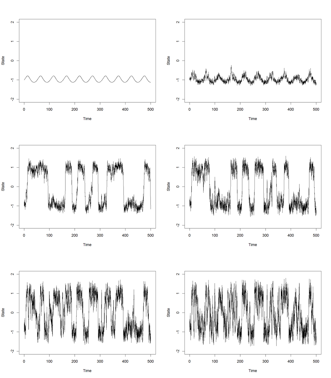
In digging through old models and scripts, I came upon one to illustrate the concept of stochastic resonance. In short, when noise is added to periodic signals with local stability, it can cause them to jump between equilibria at about the dominant frequency:
We are always looking for interesting statistical phenomena like this for models in computational psychiatry, where symptoms of mania or depression, for example, are often episodic and make large, spontaneous leaps after periods of relative stability.
The above example was produced by the following nonlinear equation with a sinusoidal force and noise term:
$$ \frac{dy(t)}{dt} = y(t)-y(t)^3 + .3\sin (.1225t) + \delta(t),\quad \delta(t) \sim N(0,1)$$
R code to generate the above animation:
library(deSolve)
dwp<-function(t, y, parms){
with(parms, {
dy<- y - y^3 + .3*sin(.35^2 * t ) + rnorm(1, 0, sigma)
return(list("dy"=dy))
})
}
Time<-500
dt<-.1
sigs<-seq(0, 5, length.out=50)
for(i in 1:length(sigs) ){
set.seed(123)
sig<-sigs[i]
x<-rk4(y=-1,t=seq(dt, Time, by=dt), dwp, parms=list("dt"=dt, "Time"=Time, "sigma"=sig))
png(paste0("stochres/",i,".png"), width=1024, height=780, pointsize = 24)
plot(x, type="l", ylim=c(-2,2), main="", xlab="Time", ylab="State")
dev.off()
}
Discretization in 3 languages
There is an obscure and useful function that makes it easy to fit stochastic differential equations to data insofar as the model can be linearized without causing too much trouble. The function discretizes the continuous-time (i.e., differential equation) state matrices A
, the drift or state transition matrix, B
, the input or covariate coefficient matrix, and Q
, diffusion or noise covariance matrix. That means that the function essentially takes the differential equation in matrix form and solves it for a given time step. The discretized matrices function like those of an autoregressive process. Some details of this approach and what this does can be found here but not exactly a complete implementation, namely with matrix B
. So this is one of those code blocks I just have backed up in several project folders in various languages.
Thanks to Mike Hunter of Georgia Tech for originally creating this and providing it in OpenMx.
R:
discretize <- function(A, B, Q, deltaT){
deltaT <- c(deltaT)
I <- diag(ncol(A))
BLOCK <- matrix(0, nrow=2*nrow(A), ncol=2*ncol(A))
# First Block expm for A integral, and expm(A*deltaT)
BLOCK[1:(2*nrow(A)), 1:ncol(A)] <- 0
BLOCK[1:nrow(A), (nrow(A)+1):(2*nrow(A))] <- I
BLOCK[(nrow(A)+1):(2*nrow(A)), (nrow(A)+1):(2*nrow(A))] <- A
BLOCK <- OpenMx::expm(BLOCK*deltaT)
expA <- BLOCK[(nrow(A)+1):(2*nrow(A)), (nrow(A)+1):(2*nrow(A))]
intA <- BLOCK[1:nrow(A), (nrow(A)+1):(2*nrow(A))]
# Second Block expm for discretized Q
BLOCK[1:(nrow(A)), 1:ncol(A)] <- -t(A)
BLOCK[(nrow(A)+1):(2*nrow(A)), 1:ncol(A)] <- 0
BLOCK[1:nrow(A), (nrow(A)+1):(2*nrow(A))] <- Q
BLOCK[(nrow(A)+1):(2*nrow(A)), (nrow(A)+1):(2*nrow(A))] <- A
BLOCK <- OpenMx::expm(BLOCK*deltaT)
Bd <- intA %*% B
Qd <- t(expA) %*% BLOCK[1:nrow(A), (nrow(A)+1):(2*nrow(A))]
return(list(Ad=expA, Bd=Bd, Qd=Qd))
}
C++ (RcppArmadillo):
// [[Rcpp::depends(RcppArmadillo)]]
#include <RcppArmadillo.h>
using namespace Rcpp;
using namespace arma;
using namespace std;
// [[Rcpp::export]]
List discretize(mat A, mat B, mat Q, double dt) {
mat M, expA, intA, Ad, Bd, Qd, I;
List output;
I.eye(A.n_rows, A.n_cols);
M.zeros(2*A.n_rows, 2*A.n_cols);
// First Block expm for A integral, and expm(A*deltaT)
M.submat(0, A.n_rows, A.n_rows-1, 2*A.n_rows-1) = I;
M.submat(A.n_rows, A.n_rows, 2*A.n_rows-1, 2*A.n_rows-1) = A;
M=expmat(M*dt);
intA = M.submat(0, A.n_rows, A.n_rows-1, 2*A.n_rows-1);
expA = M.submat(A.n_rows, A.n_rows, 2*A.n_rows-1, 2*A.n_rows-1);
// Second Block expm for discretized Q
M.submat(0, 0, A.n_rows-1, A.n_rows-1) = -1*A.t();
M.submat(A.n_rows, 0, 2*A.n_rows-1, A.n_rows-1) = zeros(A.n_rows, A.n_cols);
M.submat(0, A.n_rows, A.n_rows-1, 2*A.n_rows-1)=Q;
M.submat(A.n_rows, A.n_rows, 2*A.n_rows-1, 2*A.n_rows-1) = A;
M=expmat(M*dt);
output("Ad")=expA;
output("Bd")=intA*B;
output("Qd")=expA.t() * M.submat(0, A.n_rows, A.n_rows-1, 2*A.n_rows-1);
return output;
}
Stan:
functions{
matrix[] discretize(matrix A, matrix B, matrix Q, real dt) {
int m = rows(A);
int n = m;
matrix[m,n] expA;
matrix[m,n] intA;
matrix[m,n] I = diag_matrix(rep_vector(1.0, m));
matrix[m,n] output[3];
// First Block expm for A integral, and expm(A*deltaT)
matrix[2*m,2*n] M = append_col(rep_matrix(0, 2*m, n), append_row(I, A));
M = matrix_exp(M*dt);
intA = block(M, 1, n+1, m, n);
expA = block(M, m+1, n+1, m, n);
// Second Block expm for discretized Q
M = append_col( append_row(-1*A', rep_matrix(0, m, n)), append_row(Q, A));
M = matrix_exp(M*dt);
output[1] = expA;
output[2] = intA*B;
output[3] = expA' * block(M, 1, n+1, m, n);
return output;
}
}
Understanding MCMC and autodifferentiation
In putting together educational materials related to Stan and posterior sampling, I remembered two good ones.
The MCMC interactive gallery is the best set of MCMC visualizations I’ve found.
Stan uses NUTS, so it has to calculate numerous gradients for each new sample and does so by autodifferentiation. I recommend this video for understanding autodiff. It helps a lot to know what Stan is doing with the model code to avoid giving it more work than necessary.
Stan: Structural Ordinal Item Response Theory with a Latent Interaction
The Non-Gaussian factor model introduces the idea of using other distributions for a factor analysis. But that code is not very generalized, and in reality we’ll tend to need something more like structural equation modeling with non-Gaussian variables.
The name for a factor model with logit-linked indicators, whether dichotomous or ordinal, is Item Response Theory. It has been used for decades to develop instruments and in particular, tests. Because of its history, factor loadings are called the “discrimination” parameters, intercepts are the item “difficulty”, and the factor scores represent each person’s “ability”.
I do not know if there’s a cool brand name for IRT where multiple latent variables go on to have structure amongst themselves. But it seems useful to establish the possibility. We are essentially talking about structural equation modeling with discrete distributions.
I wrote a model to explore a number of difficult computing challenges related to that pursuit and common to the kinds of analysis requests that I get:
- Non-Gaussian factor indicators
- of which there are a large number (»20) arising from questionnaire data,
- each having 5 or more response categories, as a common property of Likert scales,
- And latent variable interactions, because everyone wants to know if their variables involve moderation.
And a bonus idea: when there are a large number of indicators and we are assuming that they function similarly in representing the factor, we can model the distribution of the factor loadings and perhaps gain a little extra power to estimate them. The discrimination parameters in IRT tend to be the least precise.
So here is a model that addresses all of that, first with simulation of the data:
D<-4 #Number of factors
Q<-50 #Indicators per factor
K<-7 #Levels per indicator
N<-600 #Sample size
z<-matrix(NA, N, D)
z[,1]<-rnorm(N)
z[,4]<-rnorm(N)
z[,2]<-rnorm(N) + .3*z[,1]
z[,3]<-rnorm(N) + 2.5*z[,1] + .3*z[,2] + 2*z[,4]*z[,1]
pairs(z)
#I know, this is actually a probit model.
dat<-array(NA, dim=c(N,D,Q))
for(d in 1:D){
for(q in 1:Q){
dat[,d,q]<- findInterval( rnorm(1,1,.05)*z[,d] + rnorm(N), seq(-1, 2, l=K-1) )+1
}
}
And then the Stan code:
functions{
}
data {
int<lower=0> N; //sample size
int<lower=1> D; //num factors
int<lower=1> Q; //num indicators per factor
int<lower=2> K; //num levels
int<lower=1,upper=K> y[N, D, Q];
}
parameters {
matrix[Q,D] lambda_z;
ordered[K-1] c[Q, D];
matrix[N,D] z;
real beta[3];
real alpha;
//optional multi-level distribution of discrimination parameters, helpful for smaller samples but many indicators
real<lower=0> lambda_mu;
real<lower=0> lambda_sd;
}
transformed parameters{
//centered parameterization for discrimination parameters
matrix[Q,D] lambda = lambda_z*lambda_sd + lambda_mu;
}
model {
z[,1] ~ std_normal();
z[,4] ~ std_normal();
z[,2] ~ normal(beta[1]*z[,1], 1.0);
z[,3] ~ normal(beta[2]*z[,1] + beta[3]*z[,2] + alpha*(z[,1].*z[,4]), 1.0);
for(d in 1:D){
for(q in 1:Q){
for(n in 1:N){
y[n, d, q] ~ ordered_logistic( z[n,d] * lambda[q, d], c[q, d]);
}
}
lambda_z[,d] ~ std_normal();
}
//optional priors
lambda_sd ~ normal(0, 5.0);
lambda_mu ~ normal(0, 5.0);
beta ~ normal(0.0,5.0);
alpha ~ normal(0.0,5.0);
}
Note certain features include grouping variables together into matrices instead of inputting them one by one, centered factor loadings (“discrimination” parameters) with a shared mean and standard deviation.
Most important for me was achievement of latent interaction by element-wise multiplication of the z-score vectors alpha*(z[,1].*z[,4])
.
No higher order moments necessary!
Stan: Non-Normal Factor Model
There are so many factor analyses in the world and so few truly normally distributed variables. I have not seen much careful tailoring of residual distributions in medical or psychological research. It is probably because most software don’t support it or make it convenient. It was a revelation to me that you can use Markov Chain Monte Carlo (MCMC) to sample latent variables and then do all kinds of things, like non-Gaussian distributions and latent variable interactions. For Stan users, this will be trivial, but I know that I would have benefited from a simple demo earlier on. So that’s what I’m posting here.
In R, a non-normal factor can be simulated this way:
f<-rnorm(n) #latent factor
x1<-rnorm(n, mean=.8*f, sd=.5)
x2<-rbinom(n, size=1, p=1/(1+exp(-2*f-.5)))
x3<-rpois(n, lambda=exp(-1 + 1.5*f))
Here is the Stan code for a simplistic model with 3 indicators distributed as normal, Bernoulli, and Poisson:
data {
int<lower=0> N;
vector[N] x1;
int x2[N];
int x3[N];
}
parameters {
real x1_mu;
real<lower=0> x1_sd;
real x2_mu;
real x3_mu;
real<lower=0> f_x1; //lower bound prevents sign indeterminacy
real<lower=0> f_x2;
real<lower=0> f_x3;
vector[N] z; //Latent variable scores- i.e., person-intercepts
}
model {
z ~ std_normal(); // N(0,1) prior for latent variables.
x1 ~ normal( x1_mu + f_x1 * z, x1_sd );
x2 ~ bernoulli( 1.0 ./( 1+exp( - f_x2 * z + x2_mu )) );
x3 ~ poisson( exp( x3_mu + f_x3 * z) );
}
Note that z
doesn’t really need to be normally distributed either.
Putting the above code in a string object model3.src
, the model is then run as follows with package rstan
:
model3<-stan_model(model_code = model3.src)
stan.dat<-list(N=n,"x1"=x1,"x2"=x2,"x3"=x3)
model3.fit<-sampling(model3, stan.dat,
iter = 1500, warmup = 500, #Reducing the amount of warmup to cut down on time.
chains=3, cores=3,
control=list(max_treedepth=8)) #Reduced treedepth from 10 to 8 to cut down time.
model3.draws<-extract(model3.fit)
Sampling z
takes a much longer time than marginalizing over it (i.e., by using matrix decomposition algebra), of course, but I do not know how to do that without assuming the indicators are normal.
And really, most of us are not using research models to shoot down missiles or dodge pedestrians, so a little extra time to do things right is worth the payoff.
Binary neural nets in R, part 2: Helmholtz Machine
github source for this project
In the last post, I looked at coding a restricted Boltzmann machine (RBM) in R. In this one, I will compare the algorithm and its results to the Helmholtz Machine, which uses the wake-sleep algorithm.
The basic idea behind the wake-sleep algorithm is that the model learns in two alternating phases. In the wake phase, random values for the hidden nodes are generated according to the expectations of the recognition network, then the generative network weights are adjusted. In the sleep phase, random values for the hidden nodes and the data are generated according to the generative network, then the recognition weights are adjusted. This process trains both the recognition and generative network, and at a good solution, the two should be nearly the same. The HM with the wake-sleep algorithm differs from the RBM in that the RBM has only one set of weights for both the top-down and bottom-up expectations for each node.
We can generate data for an HM the same way as the RBM, first by setting up a list L
with the model structure:
> L
[[1]]
[1] "bias"
[[2]]
[1] "x1" "x2" "x3" "x4" "x5" "x6" "x7" "x8" "x9" "x10" "x11" "x12" "x13" "x14" "x15" "x16" "x17" "x18" "x19" "x20"
[[3]]
[1] "h1_1" "h1_2" "h1_3" "h1_4" "h1_5" "h1_6" "h1_7" "h1_8"
Then I used a single adjacency matrix for the entire generative model, Wg
, so that I can repeatedly the same matrix multiplication, using L
to subset the result each time:
rRBM <- function(n, Wg) {
X<-matrix(0, n, ncol(Wg), dimnames=list(NULL,colnames(Wg)) )
X[,1]<-1
for(i in Q:2 ){
X[, L[[i]] ] <- (X %*% t(Wg))[, L[[i]] ]
X[, L[[i]] ] <- matrix( rbinom(prod(dim(X[, L[[i]] ])), size=1, c(lgt(X[, L[[i]] ])) ),dim(X[, L[[i]] ])[1],dim(X[, L[[i]] ])[2] )
}
return(X)
}
The wake-sleep algorithm code is given here, first with the wake phase, using Wr
to generate node values from the bottom up:
for(iter in 1:maxIter){
dat.chunk<-dat[sample(1:nrow(dat), size=chunkSize, replace=FALSE),]
X[,L[[2]]]<-dat.chunk
lr<-lr.s*temp[iter]
for(i in 3:Q){
X[, L[[i]] ] <- lgt(X %*% t(Wr))[, L[[i]] ]
X[, L[[i]] ] <- matrix( rbinom(prod(dim(X[, L[[i]] ])), size=1, c(X[, L[[i]] ]) ),dim(X[, L[[i]] ])[1],dim(X[, L[[i]] ])[2] )
}
X.p <- lgt(X %*% t(Wg))
X.p[,1]<-1
Wg.gr<- t((t(X)%*%(X-X.p))/nrow(X))
Wg[Wg.f]<- Wg[Wg.f] + lr*Wg.gr[Wg.f]
Then the sleep phase, using Wg
to generate node values from the top-down:
X2<-X
for(i in Q:2 ){
X2[, L[[i]] ] <- lgt(X2 %*% t(Wg))[, L[[i]] ]
X2[, L[[i]] ] <- matrix( rbinom(prod(dim(X2[, L[[i]] ])), size=1, c(X2[, L[[i]] ]) ),dim(X2[, L[[i]] ])[1],dim(X2[, L[[i]] ])[2] )
}
X.p <- lgt(X2 %*% t(Wr))
X.p[,1]<-1
Wr.gr<- t((t(X2)%*%(X2-X.p))/nrow(X2))
Wr[Wr.f]<- Wr[Wr.f] + lr*Wr.gr[Wr.f]
Note that both use the same local delta rule to obtain the gradient. It is computed as the the outer product of the observed and predicted values.
Here are the some results from an initial run with the same dimensions as the RBM, again looking at a redacted (|r|>.7 only) correlation matrix of the data-generating weights with the estimated weights:
Iteration 61900
Learning rate: 0.3
Hidden Layer 1 and 2 weight vector correlations: 0.3
bias h1_1 h1_2 h1_3 h1_4 h1_5 h1_6 h1_7 h1_8
bias
h1_1 -0.78
h1_2 0.98
h1_3 -0.99
h1_4
h1_5 0.99
h1_6 0.99
h1_7 0.99
h1_8 -0.99
h2_1 h2_2 h2_3 h2_4
h2_1 -0.8
h2_2 -0.83
h2_3
h2_4 -0.76
Note that I had to use the first matrix to depermute the first hidden layer in order to calculate the correlations for the second hidden layer. It’s missing one node on both accounts, but pretty cool to see both layers recovering the data-generating weights as promised! Since the learning is stochastic, it will (in theory) learn those last couple weight vectors in the course of eternity.
I increased the complexity of the simulated data and the model, then left it running for a much longer time. It looks like it was pretty successful:
Iteration 900000
Learning rate: 0.1
Hidden Layer 1 and 2 weight vector correlations: 0.1
bias h1_1 h1_2 h1_3 h1_4 h1_5 h1_6 h1_7 h1_8 h1_9 h1_10 h1_11 h1_12 h1_13 h1_14 h1_15 h1_16 h1_17 h1_18 h1_19 h1_20 h1_21 h1_22 h1_23 h1_24 h1_25 h1_26 h1_27 h1_28 h1_29 h1_30
bias
h1_1 0.98
h1_2 0.93
h1_3 -0.99
h1_4 -0.99
h1_5 0.99
h1_6 -0.99
h1_7 -0.97
h1_8 0.98
h1_9 0.98
h1_10
h1_11 0.98
h1_12 0.95
h1_13 -0.83
h1_14 -0.96
h1_15 0.98
h1_16 0.97
h1_17 -0.96
h1_18
h1_19 -0.95
h1_20 -0.98
h1_21 0.98
h1_22 -0.96
h1_23 -0.98
h1_24 0.97
h1_25 -0.96
h1_26 -0.97
h1_27 0.93
h1_28 -0.93
h1_29 0.98
h1_30 0.97
h2_1 h2_2 h2_3 h2_4 h2_5 h2_6 h2_7 h2_8
h2_1 -0.94
h2_2 0.87
h2_3 0.89
h2_4 0.89
h2_5 0.8
h2_6 0.96
h2_7 -0.93
h2_8 0.78
Painting a harpsichord lid
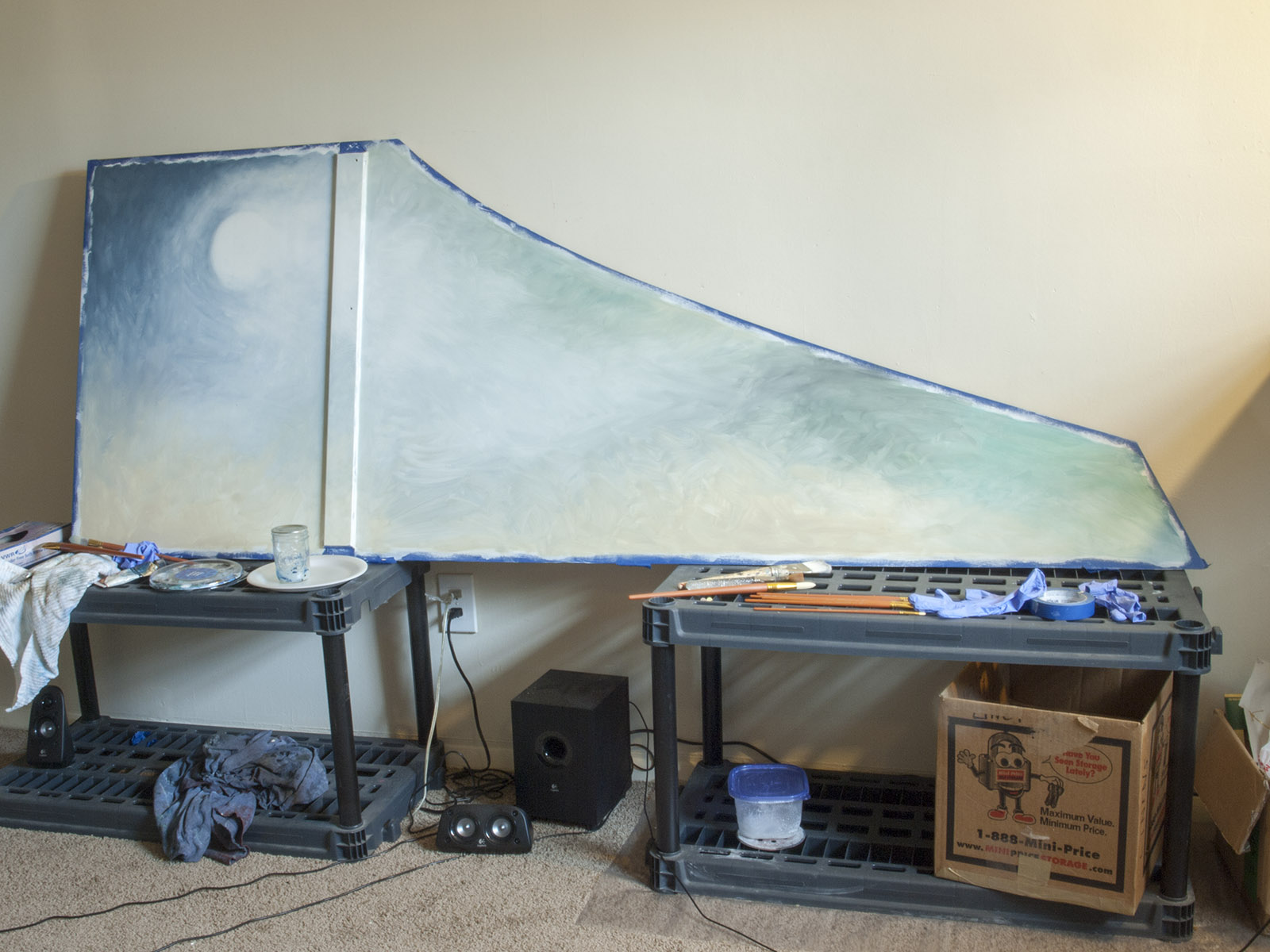
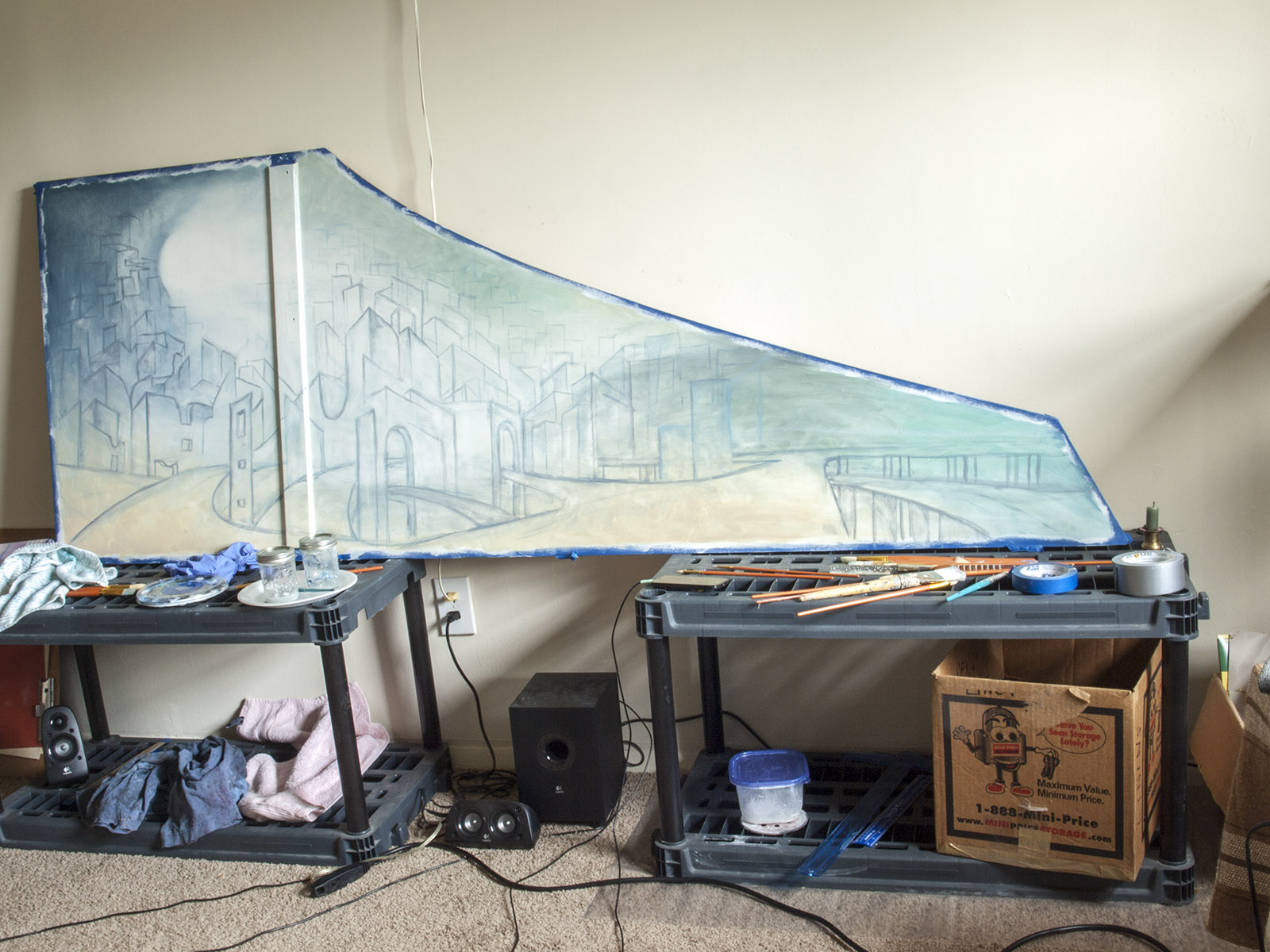
Some process photos from my painting on a harpsichord lid. (I’m using this post to figure out getting images into blog posts and such.)
I painted this harpsichord lid for a commission in 2016. I started with a photoshop mockup:
The first stages of the actual painting are interesting to look back on because they show how fundamental color and movement are to the composition:
Final result: