Binary neural nets in R, part 3: Recurrent Helmholtz Machine

github repository for this project

Part 3 of my neural network project in R involves coding a recurrent version of the Helmholtz machine. A recurrent (i.e., autoregressive or time-lagged) version of the network follows naturally (kind of), and of course, Hinton already published the idea in 1995. I used his paper as a guide to be sure nothing was markedly different about the approach and coded it according to my previous strategy.

This graphic should help understand the difference in model structure, with the top two indicating the recognition (left) and generation (right) networks of a basic Helmholtz machine, simplified to one node per layer:

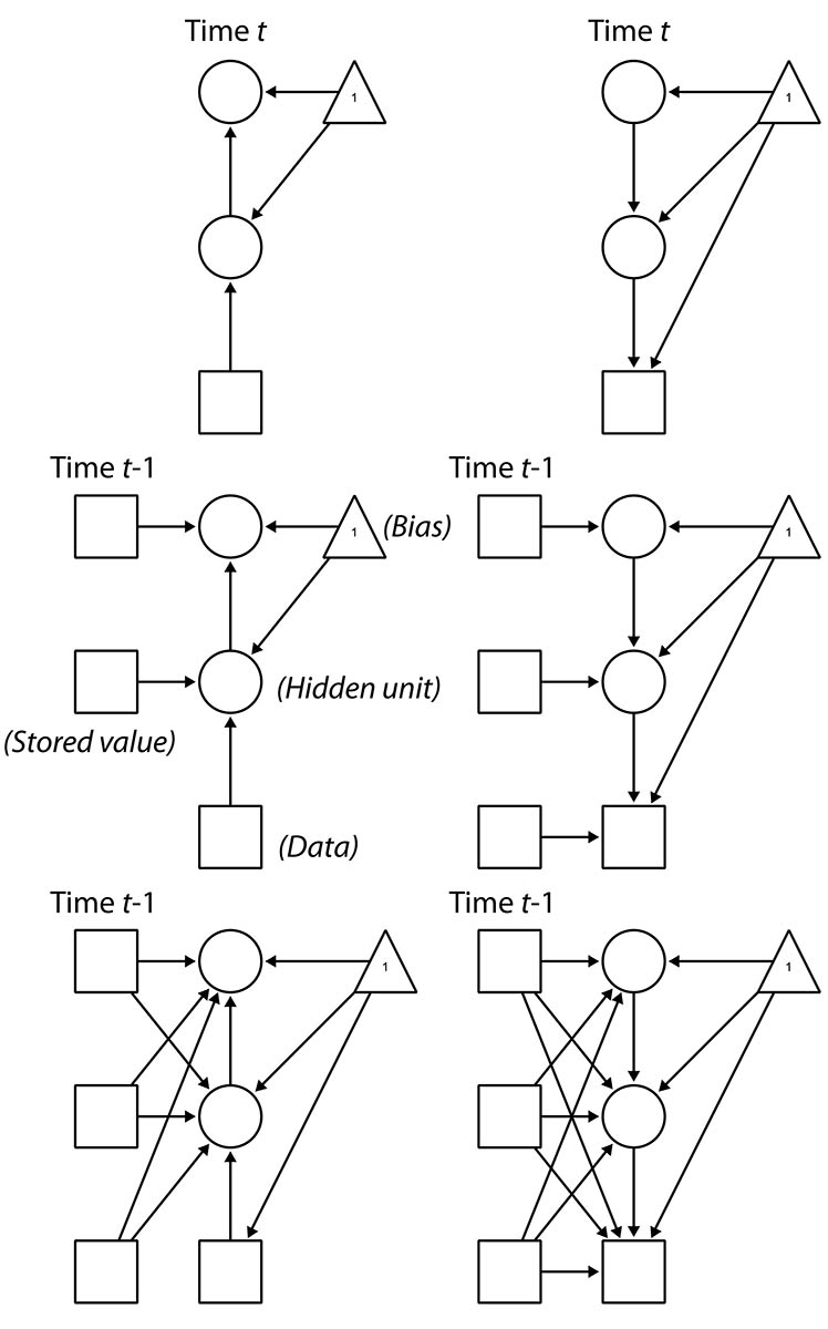
The center row figures show the addition of recurrent elements by storing the last set of hidden node values as fixed. Notice that not only are they fixed, but they are not generated in the sleep phase of learning. Because of this, we can also go on to specify the model in the third row, where all current layers draw from all stored lags. The effect is something akin to both lateral connectivity within-layer and connections that can skip layers.

One unexplored thought is that of un-fixed lagged values of the hidden nodes in the generative (i.e., sleep) phase. What would it mean for learning and recall if the model can “dream” retroactively? Memories in the human brain are not necessarily fixed. Every new recollection of a memory alters it slightly and some memories can be highly distorted by suggestion. In dreams, it’s common to experience a sense of continuity from before the moment of experience or even exact false memories that rationalize what is happening in the dream. I suppose a sensible configuration to try would be to fix the stored values of the observed data but allow past values of hidden nodes at higher layers to be re-evaluated with the addition of new information.

For now, I’ll keep it as simple as possible and let all lagged values remain fixed. To get started, I changed the list L to have another level of depth, allowing time lags, as hinted by the additional subscript on the variable names _l0_l3: For 2 hidden layers of dimension 8 and 4, each with 3 lags, we get:

[[1]]
[1] "bias"

[[2]]
[[2]][[1]]
 [1] "x1_l0"  "x2_l0"  "x3_l0"  "x4_l0"  "x5_l0"  "x6_l0"  "x7_l0"  "x8_l0"  "x9_l0"  "x10_l0" "x11_l0" "x12_l0"

[[2]][[2]]
 [1] "x1_l1"  "x2_l1"  "x3_l1"  "x4_l1"  "x5_l1"  "x6_l1"  "x7_l1"  "x8_l1"  "x9_l1"  "x10_l1" "x11_l1" "x12_l1"

[[2]][[3]]
 [1] "x1_l2"  "x2_l2"  "x3_l2"  "x4_l2"  "x5_l2"  "x6_l2"  "x7_l2"  "x8_l2"  "x9_l2"  "x10_l2" "x11_l2" "x12_l2"

[[2]][[4]]
 [1] "x1_l3"  "x2_l3"  "x3_l3"  "x4_l3"  "x5_l3"  "x6_l3"  "x7_l3"  "x8_l3"  "x9_l3"  "x10_l3" "x11_l3" "x12_l3"


[[3]]
[[3]][[1]]
[1] "h1_n1_l0" "h1_n2_l0" "h1_n3_l0" "h1_n4_l0" "h1_n5_l0" "h1_n6_l0" "h1_n7_l0" "h1_n8_l0"

[[3]][[2]]
[1] "h1_n1_l1" "h1_n2_l1" "h1_n3_l1" "h1_n4_l1" "h1_n5_l1" "h1_n6_l1" "h1_n7_l1" "h1_n8_l1"

[[3]][[3]]
[1] "h1_n1_l2" "h1_n2_l2" "h1_n3_l2" "h1_n4_l2" "h1_n5_l2" "h1_n6_l2" "h1_n7_l2" "h1_n8_l2"

[[3]][[4]]
[1] "h1_n1_l3" "h1_n2_l3" "h1_n3_l3" "h1_n4_l3" "h1_n5_l3" "h1_n6_l3" "h1_n7_l3" "h1_n8_l3"


[[4]]
[[4]][[1]]
[1] "h2_n1_l0" "h2_n2_l0" "h2_n3_l0" "h2_n4_l0"

[[4]][[2]]
[1] "h2_n1_l1" "h2_n2_l1" "h2_n3_l1" "h2_n4_l1"

[[4]][[3]]
[1] "h2_n1_l2" "h2_n2_l2" "h2_n3_l2" "h2_n4_l2"

[[4]][[4]]
[1] "h2_n1_l3" "h2_n2_l3" "h2_n3_l3" "h2_n4_l3"

The generative and recognition adjacency weight matrices Wg and Wr now include columns and rows for all of the above labels, so the dimensionality grows quite quickly. This is where R’s slowness makes it difficult to really evaluate this model. My work is ahead of me to implement it in Python.

Anyways, the wake-sleep cycle is mostly the same. The bottom-up and top-down expectations have many more terms from the lagged values, but my single-matrix approach easily generalizes to allow for that. There is however extra code appending the matrix of complete node values to store those generated at each iteration in the previous row:

    if(t>1) for(l in 1:min(t-1,lags) ) X[t,unlist(lapply(L[-1],"[",l+1))]<-X[t-l,unlist(lapply(L[-1],"[",1))]

This is added to the beginning of each loop that calculates the layer expectations.

#Start values
Wg[Wg.f]<-rnorm(sum(Wg.f))
Wr[Wr.f]<-rnorm(sum(Wr.f))


Wr[Wr==1]<-0
Wg[Wg==1]<-0

nIter<- 500000
for(i in 1:nIter){
  # X.gen<-rRHH(n+1, sim.Wg)[-1,]
  # dat<-X.gen[,unlist(L[[2]][[1]])]
  dat.chunk.seg<-sample(1:(nrow(dat.bit)-chunkSize), size=1 )
  dat.chunk<-dat.bit[dat.chunk.seg:(dat.chunk.seg+chunkSize-1),]
  
  n<-chunkSize
  
  X<-matrix(0, n, dim.total, dimnames=list(NULL, dim.v))
  X[,1]<-1
  X[,unlist(L[[2]][[1]]) ]<-as.matrix(dat.chunk)
  
  
#WAKE
  for(t in 1:n){
    if(t>1) for(l in 1:min(t-1,lags) ) X[t,unlist(lapply(L[-1],"[",l+1))]<-X[t-l,unlist(lapply(L[-1],"[",1))]
    x<-as.matrix(X[t,])
    for(h in 3:Q){
      x[L[[h]][[1]],]<-lgt(Wr%*%x)[L[[h]][[1]],]
      x[L[[h]][[1]],]<-rbinom(length(x[L[[h]][[1]]]), 1, x[L[[h]][[1]],] )
    }
    X[t,unlist(lapply(L,"[",1))]<-t(x[unlist(lapply(L,"[",1)),])
  }
  
   X.p<-lgt(X%*%t(Wg))
   X.p[,1]<-1
   Wg.gr<-t((t(X)%*%(X-X.p))/nrow(X))
   Wg[Wg.f]<- (Wg + lr*Wg.gr)[Wg.f]
  
    
#SLEEP
   X<-matrix(0, n, dim.total, dimnames=list(NULL, dim.v))
   X[,1]<-1
   for(t in 1:n){
     if(t>1) for(l in 1:min(t-1,lags) ) X[t,unlist(lapply(L[-1],"[",l+1))]<-X[t-l,unlist(lapply(L[-1],"[",1))]
     x<-as.matrix(X[t,])
     for(h in Q:2){
       x[L[[h]][[1]],]<-lgt(Wg%*%x)[L[[h]][[1]],]
       x[L[[h]][[1]],]<-rbinom(length(x[L[[h]][[1]]]), 1, x[L[[h]][[1]],] )
     }
     X[t,unlist(lapply(L,"[",1))]<-t(x[unlist(lapply(L,"[",1)),])
     
   }
  
    
   X.p<-lgt(X%*%t(Wr))
   X.p[,1]<-1
   Wr.gr<-t((t(X)%*%(X-X.p))/nrow(X))
   Wr[Wr.f]<-(Wr + lr*Wr.gr)[Wr.f]
   
   if(i%%5==0) cat("\r",i,"\t\t")
   
   #Output 
   if(i%%150==0){
     cat("\nData:\t")
     print(printData(dat.chunk))
     cat("\nSleep output:\t")
     print(printData(X[,L[[2]][[1]]]))
     cat("\nSimulation:\t")
     print(printData(rRHH(20, Wg)[,L[[2]][[1]]]))
     cat("\n\n")
   }
}

I am training this model on the Wikipedia page for the American civil war. I mapped every word to a binary vector, so it can just learn successions of them:

dat<-read.csv("textData.csv", sep=" ", header=FALSE)[,1]
p<-ceiling(log2(length(unique(dat))))
bitMap<-expand.grid(rep( list(0:1), p))[1:length(unique(dat)),]
rownames(bitMap)<-sort(unique(dat))
dat.bit<-bitMap[dat,]

Here are some simulations from 209000 iterations of model dimension c(10,8,6,4) with 5 lags.

Simulation:	[1] "NA jeb control tired results bay wagner ( the 112 the presidency newly enthusiasm towards the ferocious forage flotilla dramatically"
Simulation:	[1] "miles off the don absolutely violent outgoing emerged were heartland north towards the 260 cover rich NA absolutely overthrow 's"
Simulation:	[1] "stationing menace destination 280 the aged religious NA NA that work otherwise militia nullify divisions produced . legal wise .["
Simulation:	[1] "homestead 15 use the comprised motivation admission were the single rank the norfolk ) fence enforcement converting the whether were"

Results so far suggest that either this is not a very effective approach to modeling language, or that the complexity is much greater than I can compute in R. I sorted the text-to-binary key in alphabetical order, so you get a lot of alternation between alphabetically adjacent words with random error. Perhaps a non-stochastic network is more sensible.

Binary neural nets in R, part 2: Helmholtz Machine

github source for this project

In the last post, I looked at coding a restricted Boltzmann machine (RBM) in R. In this one, I will compare the algorithm and its results to the Helmholtz Machine, which uses the wake-sleep algorithm.

The basic idea behind the wake-sleep algorithm is that the model learns in two alternating phases. In the wake phase, random values for the hidden nodes are generated according to the expectations of the recognition network, then the generative network weights are adjusted. In the sleep phase, random values for the hidden nodes and the data are generated according to the generative network, then the recognition weights are adjusted. This process trains both the recognition and generative network, and at a good solution, the two should be nearly the same. The HM with the wake-sleep algorithm differs from the RBM in that the RBM has only one set of weights for both the top-down and bottom-up expectations for each node.

We can generate data for an HM the same way as the RBM, first by setting up a list L with the model structure:

> L
[[1]]
[1] "bias"

[[2]]
 [1] "x1"  "x2"  "x3"  "x4"  "x5"  "x6"  "x7"  "x8"  "x9"  "x10" "x11" "x12" "x13" "x14" "x15" "x16" "x17" "x18" "x19" "x20"

[[3]]
[1] "h1_1" "h1_2" "h1_3" "h1_4" "h1_5" "h1_6" "h1_7" "h1_8"

Then I used a single adjacency matrix for the entire generative model, Wg, so that I can repeatedly the same matrix multiplication, using L to subset the result each time:

rRBM <- function(n, Wg) {
  X<-matrix(0, n, ncol(Wg), dimnames=list(NULL,colnames(Wg)) )
  X[,1]<-1
  for(i in Q:2 ){
    X[, L[[i]] ] <- (X %*% t(Wg))[, L[[i]] ]
    X[, L[[i]] ] <- matrix( rbinom(prod(dim(X[, L[[i]] ])), size=1, c(lgt(X[, L[[i]] ])) ),dim(X[, L[[i]] ])[1],dim(X[, L[[i]] ])[2] )
  }
  return(X)
}

The wake-sleep algorithm code is given here, first with the wake phase, using Wr to generate node values from the bottom up:

for(iter in 1:maxIter){
  dat.chunk<-dat[sample(1:nrow(dat), size=chunkSize, replace=FALSE),]
  X[,L[[2]]]<-dat.chunk

  lr<-lr.s*temp[iter]
  for(i in 3:Q){
    X[, L[[i]] ] <- lgt(X %*% t(Wr))[, L[[i]] ]
    X[, L[[i]] ] <- matrix( rbinom(prod(dim(X[, L[[i]] ])), size=1, c(X[, L[[i]] ]) ),dim(X[, L[[i]] ])[1],dim(X[, L[[i]] ])[2] )
  }
  X.p <- lgt(X %*% t(Wg))
  X.p[,1]<-1
  Wg.gr<- t((t(X)%*%(X-X.p))/nrow(X))
  Wg[Wg.f]<- Wg[Wg.f]  +  lr*Wg.gr[Wg.f]

Then the sleep phase, using Wg to generate node values from the top-down:

  X2<-X
  for(i in Q:2 ){
    X2[, L[[i]] ] <- lgt(X2 %*% t(Wg))[, L[[i]] ]
    X2[, L[[i]] ] <- matrix( rbinom(prod(dim(X2[, L[[i]] ])), size=1, c(X2[, L[[i]] ]) ),dim(X2[, L[[i]] ])[1],dim(X2[, L[[i]] ])[2] )
  }
  X.p <- lgt(X2 %*% t(Wr))
  X.p[,1]<-1
  Wr.gr<- t((t(X2)%*%(X2-X.p))/nrow(X2))
  Wr[Wr.f]<- Wr[Wr.f]  +  lr*Wr.gr[Wr.f]

Note that both use the same local delta rule to obtain the gradient. It is computed as the the outer product of the observed and predicted values.

Here are the some results from an initial run with the same dimensions as the RBM, again looking at a redacted (|r|>.7 only) correlation matrix of the data-generating weights with the estimated weights:

Iteration 61900 

Learning rate: 0.3 

Hidden Layer 1 and 2 weight vector correlations: 0.3 
     bias h1_1 h1_2  h1_3  h1_4  h1_5 h1_6 h1_7 h1_8
bias                                                
h1_1                -0.78                           
h1_2      0.98                                      
h1_3                      -0.99                     
h1_4                                                
h1_5           0.99                                 
h1_6                                            0.99
h1_7                                  0.99          
h1_8                            -0.99               
     h2_1  h2_2 h2_3  h2_4
h2_1            -0.8      
h2_2                 -0.83
h2_3                      
h2_4      -0.76           

Note that I had to use the first matrix to depermute the first hidden layer in order to calculate the correlations for the second hidden layer. It’s missing one node on both accounts, but pretty cool to see both layers recovering the data-generating weights as promised! Since the learning is stochastic, it will (in theory) learn those last couple weight vectors in the course of eternity.

I increased the complexity of the simulated data and the model, then left it running for a much longer time. It looks like it was pretty successful:

Iteration 900000 

Learning rate: 0.1 

Hidden Layer 1 and 2 weight vector correlations: 0.1 
      bias h1_1  h1_2 h1_3 h1_4  h1_5 h1_6 h1_7  h1_8  h1_9 h1_10 h1_11 h1_12 h1_13 h1_14 h1_15 h1_16 h1_17 h1_18 h1_19 h1_20 h1_21 h1_22 h1_23 h1_24 h1_25 h1_26 h1_27 h1_28 h1_29 h1_30
bias                                                                                                                                                                                     
h1_1                                                                                                               0.98                                                                  
h1_2                                                                                                                                                         0.93                        
h1_3                                                                                                                                -0.99                                                
h1_4                                                                                                                                                              -0.99                  
h1_5                                       0.99                                                                                                                                          
h1_6                                                  -0.99                                                                                                                              
h1_7                                                                                                        -0.97                                                                        
h1_8                                                                           0.98                                                                                                      
h1_9                  0.98                                                                                                                                                               
h1_10                                                                                                                                                                                    
h1_11                                                                                                                                      0.98                                          
h1_12      0.95                                                                                                                                                                          
h1_13                                                             -0.83                                                                                                                  
h1_14                                                                                           -0.96                                                                                    
h1_15                                                                                                                                                  0.98                              
h1_16                                                                                                                                                                          0.97      
h1_17           -0.96                                                                                                                                                                    
h1_18                                                                                                                                                                                    
h1_19                                           -0.95                                                                                                                                    
h1_20                                                                               -0.98                                                                                                
h1_21                                                                    0.98                                                                                                            
h1_22                                                       -0.96                                                                                                                        
h1_23                           -0.98                                                                                                                                                    
h1_24                                                                                                                          0.97                                                      
h1_25                                                                                                                                           -0.96                                    
h1_26                                                                                                 -0.97                                                                              
h1_27                                                                                                                                                                                0.93
h1_28                                                                                     -0.93                                                                                          
h1_29                      0.98                                                                                                                                                          
h1_30                                                                                                                                                                    0.97            
     h2_1 h2_2 h2_3 h2_4  h2_5 h2_6  h2_7 h2_8
h2_1                     -0.94                
h2_2      0.87                                
h2_3                           0.89           
h2_4                0.89                      
h2_5                                       0.8
h2_6           0.96                           
h2_7                                -0.93     
h2_8 0.78